Horizontal Control
A good rule of thumb is to verify the integrity of the horizontal control by observing baselines between these stations first. The vectors can be used to both corroborate the accuracy of the published coordinates and later to resolve the scale, shift, and rotation parameters between the control positions and the new network that will be determined by GPS/GNSS. These baselines are frequently the longest in the project, and there is an added benefit to measuring them first. By processing a portion of the data collected on the longest baselines early in the project, the most appropriate length of the subsequent sessions can be found. This test may allow improvement in the productivity on the job without erosion of the final positions. By observing the horizontal control baselines first, you can discover any difficulty with the published coordinates. For example, if they are NGS brass caps, you would learn if there is any discrepancy with the published coordinates on these control stations.
Julian Day in Naming Sessions
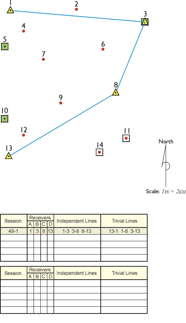
The table in the illustration indicates that the name of the first session connecting the horizontal control is 49-1. The date of the planned session is given in the Julian system. Taken most literally, Julian dates are counted from January 1, 4713 B.C. However, most practitioners of GPS/GNSS use the term to mean the day of the current year measured consecutively from January 1. Under this construction, since there are 31 days in January, Julian day 49 is February 18. The designation 49-1 means that this is to be the first session on that day. Some prefer to use letters to distinguish the session. In that case, the label would be 49-A.
Independent Lines
This project will be done with four receivers. The table shows that receiver A will occupy point 1; receiver B, point 3; receiver C, point 8; and receiver D, point 13 in the first session. Where r is the number of receivers, every session yields r-1 independent baselines. That is why the illustration shows only three of the possible six base lines that will be produced by this arrangement. Only the independent, also known as nontrivial, lines are shown on the map. The three lines that are not drawn are called trivial, and are also known as dependent lines. This idea is based on restricting the use of the lines created in each observing session to the absolute minimum needed to produce a unique solution. In the planning stage, it is best to consider the shortest vectors independent and the three longest lines are eliminated as trivial, or dependent. That is the case with the session illustrated but it cannot be said that the shortest lines are always chosen to be the independent lines. Sometimes, there are reasons to reject one of the shorter vectors due to incomplete data, cycle slips, multipath, or some other weakness in the measurements. Before such decisions can be made, each session will require analysis after the data has actually been collected.
Another aspect of the distinction between independent and trivial lines involves the concept of error of closure, or loop closure. Loop closure is a procedure by which the internal consistency of a GPS/GNSS network is discovered. A series of baseline vector components from more than one GPS/GNSS session, forming a loop or closed figure, is added together. The closure error is the ratio of the length of the line representing the combined errors of all the vector’s components to the length of the perimeter of the figure. Any loop closures that only use baselines derived from a single common GPS/GNSS session will yield an apparent closure error of zero, because they are derived from the same simultaneous observations. For example, all the baselines between the four receivers in session 49-1 of the illustrated project will be based on ranges to the same GPS/GNSS satellites over the same period of time. Therefore, the trivial lines of 13- 1, 1-8, and 3-13 will be derived from the same information used to determine the independent lines of 1-3, 3-8, and 8-13. It follows that, if the fourth line from station 13 to station 1 were included to close the figure of the illustrated session, the error of closure would be zero. The same may be said of the inclusion of any of the trivial lines. Their addition cannot add any redundancy or any geometric strength to the lines of the session, because they are all derived from the same data. If redundancy cannot be added to a GPS/GNSS session by including any more than the minimum number of independent lines, how can the baselines be checked? Where does redundancy in GPS/GNSS work come from?
Redundancy
Redundancy means stations being measured more than once. It is a useful thing in trying to evaluate the accuracy or the correctness of a network.
If only two receivers were used to complete the illustrated project, there would be no trivial lines and it might seem there would be no redundancy at all. But to connect every station with its closest neighbor, each station would have to be occupied at least twice, and each time during a different session. For example, with receiver A on station 1 and receiver B on station 2, the first session could establish the baseline between them. The second session could then be used to measure the baseline between station 1 and station 4. It would certainly be possible to simply move receiver B to station 4 and leave receiver A undisturbed on station 1. However, some redundancy could be added to the work if receiver A were reset. If it were re-centered, re-plumbed, and its H.I. (height of instrument) re-measured, some check on both of its occupations on station 1 would be possible when the network was completed. Under this scheme, a loop closure at the end of the project would have some meaning. If one were to use such a scheme on the illustrated project and connect into one loop all of the 14 baselines determined by the 14 two-receiver sessions, the resulting error of closure would be useful. It could be used to detect blunders in the work, such as mis-measured H.I.s. Such a loop would include many different sessions. The ranges between the satellites and the receivers defining the baselines in such a circuit would be from different constellations at different times. On the other hand, if it were possible to occupy all 14 stations in the illustrated project with 14 different receivers simultaneously and do the entire survey in one session, a loop closure would be absolutely meaningless.
As soon as three or more receivers are considered, the discussion of redundant measurement must be restricted to independent baselines, excluding trivial lines. In the real world, such a project is not done with 14 receivers nor with 2 receivers, but with 3, 4, or 5. The achievement of redundancy takes a middle road. Redundancy is then defined by the number of independent baselines that are measured more than once, as well as by the percentage of stations that are occupied more than once. While it is not possible to repeat a baseline without reoccupying its endpoints, it is possible to reoccupy a large percentage of the stations in a project without repeating a single baseline. These two aspects of redundancy in GPS/GNSS - the repetition of independent baselines and the reoccupation of stations - are somewhat separate.
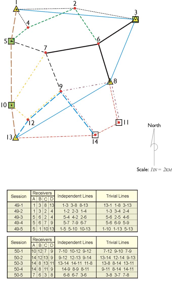
The illustration above shows one of the many possible approaches to setting up the baselines for this particular GPS/GNSS project. The design in the illustration shows lines in different colors showing the occupations using four GPS/GNSS receivers and how they are used through simultaneous occupation on these stations to create a network. The session numbers are in the table, the independent and trivial lines are listed. The A, B, C, and D receivers are shown and what points they occupy, at what stages. This is obviously done over 10 sessions over two consecutive days, and there's a good deal of redundancy in the network. However, that's simply the design. That doesn't mean that that's what will actually occur.
The survey design calls for the horizontal control to be occupied in session 49-1. It is to be followed by measurements between two control stations and the nearest adjacent project points in session 49-2. As shown in the table at the bottom of the figure, there will be redundant occupations on stations 1 and 3. Even though the same receivers will occupy those points, their operators will be instructed to reset them at a different H.I.s for the new session. A better, but probably less efficient, plan would be to occupy these stations with different receivers than were used in the first session.
Forming Loops
As the baselines are drawn on the project map for a static GPS/GNSS survey, or any GPS/GNSS work where accuracy is the primary consideration, the designer should remember that part of their effectiveness depends on the formation of complete geometric figures. When the project is completed, these independent vectors should be capable of formation into closed loops that incorporate baselines from two to four different sessions. In the illustrated baseline plan, no loop contains more than ten vectors, no loop in more than 100 km long, and every observed baseline will have a place in a closed loop.
Ties to the Vertical Control
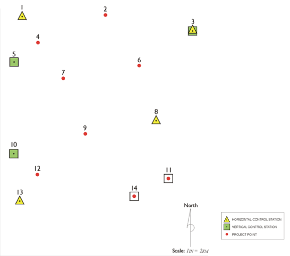
The ties from the vertical control stations to the overall network are usually not handled by the same methods used with the horizontal control. The first session of the illustrated project was devoted to occupation of all the horizontal control stations. There is no similar method with the vertical control stations. First, the geoidal undulation would be indistinguishable from baseline measurement error. Second, the primary objective in vertical control is for each station to be adequately tied to its closest neighbor in the network. If a benchmark can serve as a project point, it is nearly always advisable to use it, as was done with stations 11 and 14 in the illustrated project. A conventional level circuit can often be used to transfer a reliable orthometric elevation from vertical control station to a nearby project point.