Introduction to a Simple Planetary Climate Model
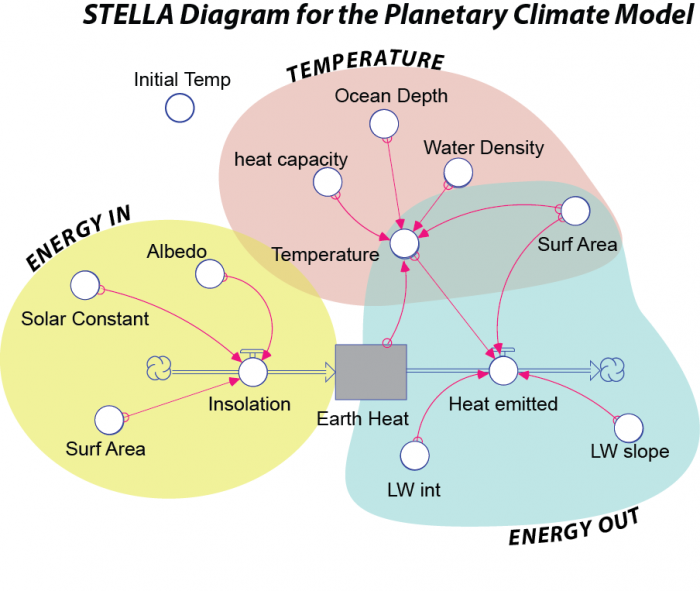
Our first model is slightly more complicated than the diagram shown above because there are quite a few other parameters that determine how much energy is received and emitted and how the temperature of the Earth relates to the amount of thermal energy stored. The complete model is shown below, with three different sectors of the model highlighted in color:
- Diagram Overview:
- A STELLA diagram titled "STELLA Diagram for the Planetary Climate Model."
- Models the energy balance and climate dynamics of Earth.
- Components:
- Reservoir: A gray box labeled "Earth Heat," representing stored thermal energy.
- Flows:
- "Insolation" (left, with a cloud symbol), flowing into the reservoir, labeled "ENERGY IN."
- "Heat emitted" (right, with a cloud symbol), flowing out of the reservoir, labeled "ENERGY OUT."
- Converters (Circles):
- Energy In (Yellow Section): Includes "Solar Constant," "Albedo," and "Surf Area," influencing "Insolation."
- Energy Out (Blue Section): Includes "LW int," "LW slope," and "Surf Area," influencing "Heat emitted."
- Temperature (Pink Section): Includes "Temperature," "heat capacity," "Ocean Depth," and "Water Density," influencing the system.
- "Initial Temp" (top left) sets the starting temperature.
- Connections:
- Pink arrows connect converters to flows and the reservoir:
- "Solar Constant," "Albedo," and "Surf Area" to "Insolation."
- "Temperature," "LW int," "LW slope," and "Surf Area" to "Heat emitted."
- "Temperature" to "Earth Heat," with feedback from "heat capacity," "Ocean Depth," and "Water Density."
- Pink arrows connect converters to flows and the reservoir:
- Interpretation:
- Models Earth's climate by balancing incoming energy (insolation) and outgoing energy (heat emitted).
- Temperature is influenced by Earth’s heat, ocean properties, and surface area, with feedback loops affecting the energy balance.
The Energy In sector (yellow above - albedo, solar constant, surf area, and insolation) controls the amount of insolation absorbed by the planet. The Solar Constant converter is a constant, as the name suggests — 1370 Watts/m2. This is then multiplied by the cross-sectional area of the Earth — this is the area that faces the Sun — giving a result in Watts (which you should recall is a measure of energy flow and is equal to Joules per second). This is then multiplied by (1 – albedo) to give the total amount of energy absorbed by our planet. In the form of an equation, this is:
S is the Solar Constant (1370 W/m2), Ax is the cross-sectional area, and a is the albedo (0.3 for Earth as a whole).
The Energy Out sector (blue above - surf area, LW int, LW slope) of the model controls the amount of energy emitted by the Earth in the form of infrared radiation. This is simply described by the Stefan-Boltzmann Law as being the surface area times the emissivity times the Stefan-Boltzmann constant times the temperature raised to the fourth power:
A is the whole surface area of the Earth, e is the emissivity, s is the Stefan-Boltzmann constant, and T is the temperature of the Earth.
The Temperature sector (brown above - water density, ocean depth, heat capacity, temp) of the model establishes the temperature of the Earth’s surface based on the amount of thermal energy stored in the Earth’s surface. In order to figure out the temperature of something given the amount of thermal energy contained in that object, we have to divide that thermal energy by the product of the mass of the object times the heat capacity of the object. Here is how it looks in the form of an equation (with units added):
Here, E is the thermal energy stored in Earth’s surface [Joules], A is the area of the planet [m2], d is the depth of the oceans involved in short-term climate change [m], ρ is the density of sea water [kg/m3] and Cp is the heat capacity of water [Joules/kg°K]. We assume water to be the main material absorbing, storing, and giving off energy in the climate system since most of Earth’s surface is covered by the oceans. The terms in the denominator of the above fraction will all remain constant during the model’s run through time — they are set at the beginning of the model and can be altered from one run to the next. This means that the only reason the temperature changes is because the energy stored changes.
The model has a few other parts to it, including the initial temperature of the Earth, which determines how much thermal energy is stored in the Earth at the beginning of the model run. There are also some converters that divide the energy received and the energy emitted by the surface area of the Earth to give a measure of the intensity of energy flow, of the flux, in terms of Watts/m2, which is a common form for expressing energy flows in climate science.
One unit of time in this model is equal to a year, but the program will actually calculate the energy flows and the temperature every 0.01 years.
Now that you have seen how the model is constructed, let’s explore it by doing some experiments. Here is the link to the model.
The First Run
What will happen to the temperature of the Earth if we run the model for 30 years with the following initial conditions:
Initial Temp = 0°C
Albedo = 0.3 (this will not change over time)
Emissivity = 1.0 (this will not change over time)
Ocean Depth = 100 m (this will not change over time)
Solar Constant = 1370 W/m2
These are the values you see when you first launch the model.
Video: Climate Model Introduction (3:22)
NARRATOR: Click on the model link. You should see a screen that looks like this, that has a graph here in the middle, that's got different pages you can toggle back and forth between. There's page 1. And then some controls for our model, including the albedo up here, the ocean depth, the emissivity, the initial temperature, and we can change the solar constant here if we want to. So, first, I'm going to run the model and just talk about what we see. So, you click the run button, here, and wait for it to execute. And then, when it's done, it'll display the results of this model run, which is going to go for 30 years here in this case. And here, it's showing us two parameters, one in magenta is the temperature, and it starts off at 0 degrees because we told it to start at zero.
Then, you can see that that temperature drops, and it continues to drop as you move along here and ends up kind of flattening off at a temperature of just about minus 18 degrees Celsius. And that's at about 30 years. Notice that when I put the cursor over one of these curves and then click on the mouse button, it'll tell me the value of that parameter. So, there I can see the temperature at any time the model run. So here, I start off at a temperature of zero, and it cooled very quickly to a temperature of minus eighteen. And that's in part because we have the emissivity here set at one and that means that this model planet has no greenhouse whatsoever. So, this is the presumed temperature of our planet if we had no greenhouse.
In this first set of experiments, we're going to have you do a couple of things. One is to change the initial temperature and see to what extent that affects the model's outcome, and then change the albedo up here, and then also change the emissivity. You can change these parameters by doing a couple of things. So, I'm just going to change the initial temperature here to, let's see, 20 degrees, like that. So, I can change it by moving that slider, or I can just click here in this box and type in whatever number I want. So, now I'm going to change it to 10. So, if I do that and then run the model, you can see what happens. It's going to start off at 10 degrees, and then it will evolve after that starting condition. So, here you can see it starts at 10, and it drops off as well.
You can restore it to the initial value here by clicking that little “U” and it does undo that change. And then, you can change the emissivity and run it, or change the albedo and run it. After you've made these changes to albedo or emissivity, you want to always click that “U” so you kind of return that value to its starting position. What we're going to do here is to kind of investigate the effects of changing initial temperature, emissivity, and albedo on the performance of this climate model, and we want to look at these things one at a time. Okay, so that's it.
Video: Sample Problem (2:38)
NARRATOR: When we ran this initial model, we saw that the temperature of our planet cooled. Here, we see it starting at 10 because that was the last initial temperature that I'd used, and it dropped from 10 to a temperature of about minus 18. Now the question is, why? Why did that happen? Let's consider a couple of things here. We clicked to page two here, we see a couple of other parameters graphed here. One is the energy flux in, so that's just the energy added to our planet in blue. And here's the energy out, the energy flux out, that's the energy leaving the Earth in the form of infrared radiation. And so, look what happens initially. Let's take the energy in to begin with, that starts off with a value of about 240 roughly, 239.
Okay, and that doesn't change at all throughout this model run. That has the same value of about 240. And the energy out instead, it starts quite high, 358 watts per meter squared. So, at the beginning of time, the planet is losing a lot more energy than it's gaining here at this blue line. And that continues until eventually, watch that energy flux out, it eventually gets down to be about 240. So, at this point in time, those two have exactly the same value, the energy in and energy out. When the energy in and the energy out have the same value, then our model is in what we call a steady state and the temperature won't change.
One thing just to note here is that each of these curves, the red, and the blue, are plotted with their own different scales on the vertical axis. And that's why out in this region here the two curves appear to be offset, but they actually have the same value here, right? So, it's just a little trick in the vertical axis that's misleading us a little bit there. So, the answer to the question of why did the planet cool is simply that, initially given its initial temperature, the energy leaving the planet was much higher than the energy coming into the planet, so the temperature has to drop.